This is a new one on me. Rogue started stalking my wife’s broccoli with garlic sauce. Nom?
Yes, nom. Weirdo.
Thursday, July 9, 2015

Tuesday, July 7, 2015
Spreading Imports Thin Does Not Mean Exchange Rates Do Not Matter
I am in the middle of a Twitter debate with J.W. Mason. The starting point for the debate is an empirical paper suggesting that real currency depreciation does not increase real exports, but a real currency appreciation decreases real exports (pdf).
Let us see if I can clarify my position that there is an implication that real currency depreciation leads to lower real imports.
Let us suppose there are 101 countries and everyone imports \$100 worth of goods from each of the 100 different partner countries, so that each country imports a total of \$10,000 worth of goods. Now suppose that my current depreciates, say, 10% so that everyone else’s currency appreciates1% 0.1%. Suppose further that a 1% 0.1% appreciation reduces exports by 0.05%.
At first blush it seems that this implies a 0.05% reduction in my imports. After all, if every partner country reduces their exports to every other country by 0.05%, then my imports must fall by 0.05%– almost too small to measure.
But this ignores the fact that my partner countries exchange rates did not appreciate with each other. When each partner loses 0.05% of exports, that partner reduces exports to me by \$5 and exports to the rest of the world by \$0. Thus, my total imports from all countries falls by \$500, or 5% of my initial imports.
Which is to say, I do not understand the position that the reduction in real imports due to depreciation is “formally correct but practically and empirically irrelevant.”
Let us suppose there are 101 countries and everyone imports \$100 worth of goods from each of the 100 different partner countries, so that each country imports a total of \$10,000 worth of goods. Now suppose that my current depreciates, say, 10% so that everyone else’s currency appreciates
At first blush it seems that this implies a 0.05% reduction in my imports. After all, if every partner country reduces their exports to every other country by 0.05%, then my imports must fall by 0.05%– almost too small to measure.
But this ignores the fact that my partner countries exchange rates did not appreciate with each other. When each partner loses 0.05% of exports, that partner reduces exports to me by \$5 and exports to the rest of the world by \$0. Thus, my total imports from all countries falls by \$500, or 5% of my initial imports.
Which is to say, I do not understand the position that the reduction in real imports due to depreciation is “formally correct but practically and empirically irrelevant.”
Monday, June 29, 2015
Glossip v. Gross: Getting the Logic Right?
If we agreed that “no woman shall ever launch a nuclear weapon” does it then follow that it is okay for a man to do so? It seems that Scalia answers in the affirmative.
Scalia (pdf):
Mind you, not once in the history of the American Republic has this Court ever suggested the death penalty is categorically impermissible. The reason is obvious: It is impossible to hold unconstitutional that which the Constitution explicitly contemplates. The Fifth Amendment provides that “[n]o person shall be held to answer for a capital… crime, unless on a presentment or indictment of a Grand Jury,” and that no person shall be “deprived of life… without due process of law.”He argues that because the Constitution says the government cannot execute unless if meets certain conditions, that the Constitution also permits it to execute so long as those conditions are met. I am willing to concede that the Founders thought that the death penalty was constitutional. And it would be one thing if the Constitution enumerated the power (”The government shall have the power to deprive a person of life withstanding due process of law.“ However, Scalia argues that the Constitution permits it to execute even if the government can find no way around some other constitutional barrier. There must always be a constitutional way for it to kill. From the Opinion of the Court (emphasis added):
Our decisions in this area have been animated in part by the recognition that because it is settled that capital punishment is constitutional, “[i]t necessarily follows that there must be a [constitutional] means of carrying it out.” Id., at 47. And because some risk of pain is inherent in any method of execution, we have held that the Constitution does not require the avoidance of all risk of pain. Ibid. After all, while most humans wish to die a painless death, many do not have that good fortune. Holding that the Eighth Amendment demands the elimination of essentially all risk of pain would effectively outlaw the death penalty altogether.From Breyer’s dissent:
The relevant legal standard is the standard set forth in the Eighth Amendment. The Constitution there forbids the “inflict[ion]” of “cruel and unusual punishments.” Amdt. 8. The Court has recognized that a “claim that punishment is excessive is judged not by the standards that prevailed in 1685 when Lord Jeffreys presided over the ‘Bloody Assizes’ or when the Bill of Rights was adopted, but rather by those that currently prevail.” Atkins v. Virginia, 536 U. S. 304, 311 (2002). Indeed, the Constitution prohibits various gruesome punishments that were common in Blackstone’s day. See 4 W. Blackstone, Commentaries on the Laws of England 369–370 (1769) (listing mutilation and dismembering, among other punishments).Notice the conflicting arguments:
- Scalia: It is constitutional, therefore there must be a constitutional means of execution.
- Breyer: If there is no constitutional means, then it is unconstitutional.
What is the Conflict Between Uninformed Priors and Gambling?
Via Noah Smith at Twitter, Deborah G. Mayo asks “What do hard-nosed Bayesians like Gelman really mean by posterior probability?” In reading the piece, I grew concerned that Mayo left out something important to Andrew Gelman.
The following example pretty well describes the issue at hand.
Suppose I ask you show me a coin from your pocket and then ask you to flip it once. If it comes up heads, are you now willing to stake \$3 for a chance to win \$4 if among the next 1,000 flips at least 500 are heads? Or do you still think the coin is fair and you expect this bet on average would lose you \$1?This illustrates the difference between an uninformed prior and a strong prior. If you began with a very weak prior– that is, prior to flipping the coin you believed the bias of the coin was equally likely to be always coming up heads as always coming up tails as anywhere in between– then you might take the bet. If on the other hand your experience is such that you do not frequently wind up with heavily biased coins in your own pocket then you might not think much of that first coin flip. I think Gelman’s point is that however useful you may find it to employ an uninformative prior to communicate science, that does not mean your personal prior is necessarily uninformed. Therefore you might not make personal decisions based on a posterior derived from an uniformed prior– or, presumably, any prior much different than your own. I am of two minds about the implications for reporting. My instinct is that biases should be made clear and so perhaps personal priors should be used in place of uniformed. On the other hand, a strong prior may greatly reduce the power of the study. If I believe that 999 of 1,000 coins yield tails 99 times out of 100, then a single flip of heads will do little to convince me that the coin is not biased toward tails. Is it really useful for me to report that I believe the coin is almost certainly biased toward tails? Is that science or opinion? It seems therefore that the likelihood– rather than the posterior– is the important scientific result of the study. In this case, the likelihood is identical to the posterior derived from the uniform prior, so there is no choice between these two. To take an example from my own research, consider the audit of the April 14, 2013 Venezuelan election. There, a very extensive audit– 53 percent of more than 39,000 voting machines– turned up zero discrepancies between the numbers on the machines and paper ballots counted by hand. What conclusions may be drawn from this result? If you have uninformed priors, this seems overwhelmingly to suggest that the election was free of any meaningful audit-detectable fraud. If you believe strongly that the election results were fraudulent in a manner detectable by the audit, then it seems more sensible that the audit itself was a fraud. That is, your conclusion respecting the election result depends on your priors regarding possible fraud in the audit as well as the election. Scientifically, the important conclusion is that the audit results were not consistent with detectable fraud.1 Coming back to the original posts, then, it seems to me that Mayo missed Gelman’s point that priors do matter. I think Gelman is suggesting that relatively uninformed priors are reasonable for the basis of scientific reporting; in going beyond a study the reader must construct their own posteriors. To whatever extent possible, apply your Bayesian inference to your own priors rather than allowing someone else to insert their own.
1 To the point that a full audit of all voting machines would change nobody’s conclusions respecting the election results.↩
Thursday, April 9, 2015
Retirement Incomes are Falling for Many Americans, Despite What AEI Wants You to Think
Acknowledgement: I thank Andrew Biggs for his assistance in replicating his numbers.
In a new paper from the American Enterprise Institute, Andrew Biggs and Sylvester Schieber argue that workers retirements are more secure financially than some suggest. In part, they point to the ratio of household assets to wage earnings for those with heads aged 45-54. While their criticisms may have some validity, there are some significant omissions that cut the other way. On balance, it is likely that most households will rely more heavily on Social Security to support their retirements than in prior years.
According to the Survey of Consumer Finances, on average household wealth for the 45-54 age group fell from 5.8 years of wages in 2007 to 4.7 in 2013. Household wealth here— consistent with Biggs and Schieber—includes the value of a home and any other real estate, plus financial wealth. Mortgages and other debt are subtracted to get this number, as seen in Figure 1.
Figure 1: Biggs and Schieber’s mean assets relative to household wage income: all 45-54 year old householders Source: Survey of Consumer Finances and author’s calculations
At 5 percent interest, this wealth could replace only 23.4 percent of current wage income compared to 28.8 percent in 2007.1
In a new paper from the American Enterprise Institute, Andrew Biggs and Sylvester Schieber argue that workers retirements are more secure financially than some suggest. In part, they point to the ratio of household assets to wage earnings for those with heads aged 45-54. While their criticisms may have some validity, there are some significant omissions that cut the other way. On balance, it is likely that most households will rely more heavily on Social Security to support their retirements than in prior years.
According to the Survey of Consumer Finances, on average household wealth for the 45-54 age group fell from 5.8 years of wages in 2007 to 4.7 in 2013. Household wealth here— consistent with Biggs and Schieber—includes the value of a home and any other real estate, plus financial wealth. Mortgages and other debt are subtracted to get this number, as seen in Figure 1.
Figure 1: Biggs and Schieber’s mean assets relative to household wage income: all 45-54 year old householders

At 5 percent interest, this wealth could replace only 23.4 percent of current wage income compared to 28.8 percent in 2007.1
Trends in the Labor Force 1999-2014: Seniors Increase Participation, Younger Workers Withdraw
In early 2000, the civilian labor force participation rate peaked at a post-war high of 67.3 percent of the population aged 16 and over. Despite flattening out in the latter part of the decade at about 66 percent, participation rates never recovered and have steadily fallen since the onset of the Great Recession. At 62.8 percent as of November 2014, labor force participation is now at its lowest level since 1978.
Some of this fall is clearly demographic. Workers are much less likely to have or search for a job once near or past retirement age, as seen in Figure 1.
Figure 1:
Thus, the aging of the baby boom generation has reduced the size of the labor force. On the other hand, retirement-age workers are participating at a much higher rate than before. In small part, this is because baby-boomers have reduced the average age of those 65 and over. However, labor force participation in the older population has been rising for some time, as seen in Figure 2.
Figure 2:
Some of this fall is clearly demographic. Workers are much less likely to have or search for a job once near or past retirement age, as seen in Figure 1.
Figure 1:
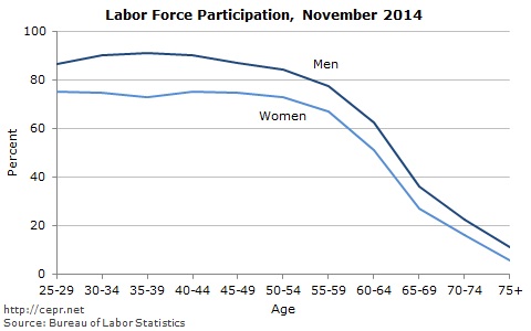
Thus, the aging of the baby boom generation has reduced the size of the labor force. On the other hand, retirement-age workers are participating at a much higher rate than before. In small part, this is because baby-boomers have reduced the average age of those 65 and over. However, labor force participation in the older population has been rising for some time, as seen in Figure 2.
Figure 2:

Tuesday, March 3, 2015
“Mumbo-Jumbo” Mumbo-Jumbo
Today, Cato’s Alan Reynolds took a few bizarre shots from the pages of the Wall Street Journal. In particular, Reynolds it calls “far-fetched” that incomes of the middle class have stagnated for decades.
First, he asserts “The average income for the bottom 90% is not a decent proxy for the median nor even a decent measure of household income." This is clearly indefensible as a check of the numbers at Reynolds’ source demonstrates. Here, we see the average of the bottom 90 percent and the median compared for both before-tax and after-tax household income.
 (Source)
Over Reynolds’ chosen 1984-2007 period, median before-tax income fell 0.05 percent per year relative to the bottom 90 percent and median after-tax income rose less than 0.01 percent per year relative to the bottom 90 percent. Obviously, such differences are in no way meaningful.
Next, Reynolds argues that median after-tax (and transfer) measures better describe the evolution of middle-class incomes than does pre-tax and transfer “market income.” However, the comparatively higher rate of growth in after-tax income simply reflects the government attempting to compensate households for the broad stagnation of income. If the median household is better off in 2007 than 23 years prior it is because we have recognized that wages have fallen and households have had to work much more to maintain a modest 0.5 percent annual increase in pre-tax income. We have increased transfers and cut taxes in order to help those households to share in the increased productivity of the economy.
It is also worth noting that much of the increased transfers which make up the wedge between market and pre-tax incomes have come as a result of a broken health-care system. The government now pays health providers considerably more and yet life expectancy for those in the bottom half of the income distribution has grown so slowly that such workers may enjoy shorter– not longer– retirements. It is not so obvious that such increases in payments contribute to growth in household income.
It is no surprise then that real per-person consumption has grown faster than median pre-tax household income. Not only does this conflate the median with the overall average— it ignores that household savings rates have declined considerably over the decades in question. In 1989, the median net wealth of households headed by someone aged 45-54 was \$177,300 compared to only \$105,400 in 2013. Even that does not consider the simultaneous decline in defined-benefit pensions held by such households.
The middle class may still appear middle class because households have dedicated more time to work, received increased assistance from the government, and accumulated considerably less wealth than the previous generations; such measures merely hide the obvious stagnation.
First, he asserts “The average income for the bottom 90% is not a decent proxy for the median nor even a decent measure of household income." This is clearly indefensible as a check of the numbers at Reynolds’ source demonstrates. Here, we see the average of the bottom 90 percent and the median compared for both before-tax and after-tax household income.

Over Reynolds’ chosen 1984-2007 period, median before-tax income fell 0.05 percent per year relative to the bottom 90 percent and median after-tax income rose less than 0.01 percent per year relative to the bottom 90 percent. Obviously, such differences are in no way meaningful.
Next, Reynolds argues that median after-tax (and transfer) measures better describe the evolution of middle-class incomes than does pre-tax and transfer “market income.” However, the comparatively higher rate of growth in after-tax income simply reflects the government attempting to compensate households for the broad stagnation of income. If the median household is better off in 2007 than 23 years prior it is because we have recognized that wages have fallen and households have had to work much more to maintain a modest 0.5 percent annual increase in pre-tax income. We have increased transfers and cut taxes in order to help those households to share in the increased productivity of the economy.
It is also worth noting that much of the increased transfers which make up the wedge between market and pre-tax incomes have come as a result of a broken health-care system. The government now pays health providers considerably more and yet life expectancy for those in the bottom half of the income distribution has grown so slowly that such workers may enjoy shorter– not longer– retirements. It is not so obvious that such increases in payments contribute to growth in household income.
It is no surprise then that real per-person consumption has grown faster than median pre-tax household income. Not only does this conflate the median with the overall average— it ignores that household savings rates have declined considerably over the decades in question. In 1989, the median net wealth of households headed by someone aged 45-54 was \$177,300 compared to only \$105,400 in 2013. Even that does not consider the simultaneous decline in defined-benefit pensions held by such households.
The middle class may still appear middle class because households have dedicated more time to work, received increased assistance from the government, and accumulated considerably less wealth than the previous generations; such measures merely hide the obvious stagnation.
Subscribe to:
Posts (Atom)