Depreciation and Income Shares

I would like now to wade briefly into a debate over the gap between growth in productivity and wages by introducing a bit of modeling fun. It seems clear that— in recent decades— although wage income has grown more slowly than GDP there has been little difference between the growth rate of NDP (GDP net of capital depreciation) and the growth rate of total labor compensation.

On the other hand, inequality of compensation has increased quite a bit— driving a large wedge between pay at the top and pay of the ordinary worker. None of this is news. Somewhat less clear is whether net product is more or less appropriate as a comparison. At first blush, workers still have to produce the whole of output no matter how much investment goes to replacing depreciating capital. It might make sense for labor compensation to rise in step with gross production. But...

Differential confusion and a note on “Standard Neoclassical pedagogy”

In my Comment to Standish and Keen, I asserted that it must be that if $P$ is defined as a function $P\!\left(Q\right)$ then it must be that ${\partial P}/{\partial q_i}$ must be zero because $P$ is not a function of $q_i$, but one of $Q$ alone. Standish and Keen wish to argue that if we hold $Q=\sum_i{q_i}$, then ${\partial P}/{\partial q_i}={dP}/{dQ}$, which is assumed to be negative. It is my contention that this may appear correct at first blush, but this compact notation masks hidden assumptions about the underlying economic model.

I tried to explain this in Section 4.2, but it appears my message was lost. Here, I am going to clarify the notation a bit. When specifying the inputs to a function, I am going to use square brackets. Evaluation of a function will employ parentheses. That is, $f\!\left[x\right]$ should be read “$f$— a function of $x$” while $f\!\left(y\right)$ should be read “$f$— a function of one variable evaluated at $y$.”

For example, though Wilfred Kaplan states in Advanced Calculus (3^rd ed.) that

If $z=f\!\left(x,y\right)$ and $x=g\!\left(u,v\right)$, $y=g\!\left(u,v\right)$, then $$ \frac{\partial z}{\partial u}=\frac{\partial z}{\partial x}\frac{\partial x}{\partial u}+\frac{\partial z}{\partial y}\frac{\partial y}{\partial u} $$

Kaplan also clarifies on the following page that $z\!\left[u,v\right]=f\!\left(g\!\left(u,v\right),h\!\left(u,v\right)\right)$ “is the function whose derivative with respect to $u$ is denoted by ${\partial z}/{\partial u}$.”

That is, when $z$ is evaluated at $\left(g\!\left(u,v\right),h\!\left(u,v\right)\right)$ the result is an entirely new function. Kaplan’s chain rule could be written more clearly (if pedantically)

If $z\!\left[x,y\right]=f\!\left(x,y\right)$ and $x\!\left[u,v\right]=g\!\left(u,v\right)$, $y\!\left[u,v\right]=h\!\left(u,v\right)$, then $$ \frac{\partial z^*\!\left[u,v\right]}{\partial u}=\frac{\partial z\!\left[x,y\right]}{\partial x}\frac{\partial x\!\left[u,v\right]}{\partial u}+\frac{\partial z\!\left[x,y\right]}{\partial y}\frac{\partial y\!\left[u,v\right]}{\partial u} $$ where $z^*\!\left[u,v\right]=z\!\left(g\!\left(u,v\right),h\!\left(u,v\right)\right)=f\!\left(g\!\left(u,v\right),h\!\left(u,v\right)\right)$

“Rationality” in the Theory of the Firm... Conclusion

Previously: Introduction; Part 1; Part 2; Part 3; Part 4; Part 5; Part 6; Part 7; Part 8

As we have seen, the response of Keen and Standish is sorely lacking. They continue to misunderstand or misrepresent textbook models, fail to recognize how competitive profit maximization lowers profits, offer no coherent theory to support their contrary arguments, and continue to insist– despite all evidence– that their simulations support their claims.

Defending this failure, the authors write

Admittedly, the agents specified in our paper are not sophisticated enough to do this, but this was a deliberate choice, since we wanted to show that agents following a simple iterative and non-collusive algorithm would choose output levels that clustered around the true profit-maximizing level of output, and not the Cournot level.

The words “not sophisticated” and “simple” are perhaps telling. Keen and Standish seem to argue that their firms are rational profit-maximizers to but insufficiently intelligent to figure out that someone else might have a better strategy. The most frustrating thing about their work is that the claim they fail to support– the existence of a competitive equilibrium at the collusive level within the infinitely-repeated Cournot-Nash game– is itself textbook. Far from debunking textbook economics, they simply do a terrible job of catching up to it.

---

Read my original Comment (including Technical Appendix) at World Economic Review.

“Rationality” in the Theory of the Firm... Part 8

Previously: Introduction; Part 1; Part 2; Part 3; Part 4; Part 5; Part 6; Part 7

Keen and Standish write

This focuses on the simple agent model we use to explore this issue. Rosnick compares the model to agents dancing in a wagon careering downhill. Whilst poetic, it is not a useful metaphor, chiefly because with the wagon, the system’s dynamics are largely determined by the trajectory of the wagon, not the individual agents, whereas with our model, the dynamic behaviour is completely determined by the actions of the agents.

Here, they misunderstand the story. Each firm is– in their simulations– out of control. The rise or fall in its profits is almost entirely determined by the actions of all its competitors and not at all its own actions. Thus, it is not rational for the firm to make decisions based on the assumption that it is in control. Much of the time a firm thinks it made a decision which raised its profits, the firm actually made the wrong choice. Much of the time a firm thinks it made a decision which lowered its profits, the firm actually made the correct choice. It is a funny kind of rationality, that.

They continue,

In §6.3, Rosnick introduces a variant of our agents where the decision is made to reverse the usual decision with small probability that increases the closer to equilibrium the system is. Undoubtedly, this could be done so as to benefit the agent concerned, to the detriment of the other agents in the system, however this action cannot be considered rational. Rational agents always choose the optimum action — the only time rational agents are permitted to act stochastically is when multiple equally valued courses of action are available.

First of all, in the strategy I laid out in this Section 6.3 the decision to reverse is based not on closeness to equilibrium, but the change in profits from the previous period. That aside, this critique cuts against Keen and Standish. Far from always choosing the “optimum action” their firms make inferior choices quite often. By their own argument, then, their agents are irrational. The whole point of a firm reconsidering is to avoid letting the rest of the industry fool it into making inferior choices. There is no reason to rule out stochastic strategies, but even if we disallowed those, chance is not required to accomplish the goal. Keen and Standish simply ignore Section 6.4 of my Comment and the entire Technical Appendix. This only points the way, of course. As discussed in Section 6.1 of my Comment and in Part 4 Keen and Standish still leave undefined the infinite-horizon utility for the firm; without knowing how the firm aggregates profits accumulated over the entire course of the game, there is no way to prove that it has employed an optimal strategy to maximize such profits.

This passage does underline the notion that Keen and Standish do not understand the theory they criticize. Agents may be allowed to choose randomly among choices to which it is indifferent. However, agents may not be indifferent between deterministic and stochastic strategies. It may certainly be that a stochastic strategy pays better than a deterministic one. It may also be that a second deterministic strategy pays even better than the stochastic strategy, but that is actually irrelevant; if any strategy pays better than the one suggested by Keen and Standish, then the equilibrium falls apart.

Most importantly, when Keen and Standish concede “this could be done so as to benefit the agent concerned, to the detriment of the other agents in the system” they concede the whole critique. If– given the strategies employed by the other firms– a superior strategy may be found, then a competitive profit-maximizing firm must use the superior strategy. How can it be rational to leave profits on the table for another firm to collect– except by agreeing with other firms that nobody will ruin their good thing by thinking of their own self-interest?

Contrary to the authors’ claim, their firms do not pursue clearly a strategy that is both rational and non-collusive. As best as may be determined in the absence of a clear objective for the full game, either firms fail to recognize that there is money on the table, or they agree with the others to leave it there.

Conclusion

---

Read my original Comment (including Technical Appendix) at World Economic Review.

“Rationality” in the Theory of the Firm... Part 7

Previously: Introduction; Part 1; Part 2; Part 3; Part 4; Part 5; Part 6

In their response, Keen and Standish propose the following dynamics:

[A]round a Keen outcome ${\bf q}^K$, we get $$ \frac{d{\bf q}}{dt}=\sum_j{\frac{\partial\pi_i}{\partial q_j}\left(q_j-q^K_j\right)} $$

Right off this math is confusing. Apparently, what they mean is $$ \frac{dq_i}{dt}=\sum_j{\frac{\partial\pi_i}{\partial q_j}\left(q_j-q^K_j\right)} $$ This suggests that they have in mind $$ {\bf F}\!\left({\bf q}\right)\equiv\boldsymbol{\pi}\!\left({\bf q}\right)-\boldsymbol{\pi}\!\left({\bf q}^K\right) $$ which, by construction yields ${d{\bf q}}/{dt}=0$ when ${\bf q}={\bf q}^K$. This much is true no matter what ${\bf q}^K$ is chosen. It is also a very strange strategy for firms to employ. Firm $i$ expands only if it has profits in excess of its benchmark profits $\pi_i\!\left({\bf q}^K\right)$, and contracts only if it has profits below its benchmark. Clearly, the symmetric collusive oligopoly is not stable according to this dynamical system. If all firms start by underproduce by some tiny amount, then they will all reduce their outputs to zero.

If marginal costs are constant, then the eigenvalues are determined by the zeroes of $$ \left|\begin{array}{cccc}\left(\lambda-P+\mathrm{MC}\right)-q_1P'&-q_1P'&\cdots&-q_1P'\\-q_2P'&\left(\lambda-P+\mathrm{MC}\right)-q_2P'&\cdots&-q_2P'\\\vdots&\vdots&\ddots&\vdots\\-q_nP'&-q_nP'&\cdots&\left(\lambda-P+\mathrm{MC}\right)-q_nP'\end{array}\right| $$ so $\lambda\in\left\{P-\mathrm{MC}+QP',P-\mathrm{MC}\right\}$. That is, profitability ($P>\mathrm{MC}$) implies instability.

Even if marginal costs are not constant, if any two firms have identical cost structures, there is no ${\bf q}$ which is both stable and symmetric. Stability is in general achieved when smaller firms are driven out of the industry and the market is monopolized by a single firm.

In Figure 1, we see 25 simulations of a duopoly ($n=2$) with costs and demand parameterized as in their earlier example. The initial output for each firm is randomly selected to be within 2 percent of the proposed equilibrium. Each simulation is seen as a line, with a marker at the end of each run– the ${\bf q}$ at time $t=0.1$ from simulation start.

Figure 1: Simulations of Keen-Standish Dynamics

Keen and Standish write

The condition describes not an equilibrium point, but rather an equilibrium manifold of constant total market production, which is stabilised by the agents ensuring that if any agent were to cause the system to stray from this manifold, then all agents will follow suit, causing that agent to not enjoy its advantage for long. Any rational agent will then return to the fold.

which is a really funny way of saying that they believe firms with higher initial production ruthlessly drive out the competition until the industry turns into a monopoly. Note that this is nothing like their earlier agent simulations in which equilibrium market shares are predictable without dependence on the initial firm choices. Keen and Standish may invoke (pdf) the movie War Games (“A strange game. The only winning move is not to play.”) but their response brings to mind Highlander. “There can be only one!”

However, the math in their response makes no sense to begin with, so the dynamical system Keen and Standish have in mind may be differ from the one analyzed above. Still, a Cournot-like strategy where firms move toward their best response to the current price such as $$ {\bf F}\!\left(q_1,q_2\right)\equiv\left[\begin{array}{c}a-c\\a-c\end{array}\right]-\left[\begin{array}{cc}2b+d&b\\b&2b+d\end{array}\right]\left[\begin{array}{c}q_1\\q_2\end{array}\right] $$ shows globally stable dynamics. Figure 2 shows this strategy simulated with each firm’s output initialized randomly to within 50 percent of the Cournot-Nash result.

Figure 2: Simulation of a Cournot-like Dynamics

This alone does not imply that either dynamic system describes optimal firm behavior; such would require still an appropriately defined firm objective such as $$ \Pi_i\!\left[{\bf q}\!\left(t\right)\right]=\int^\infty_0{\rho^t\pi_i\!\left[{\bf q}\!\left(t\right)\right]dt} $$ Rather, the examples demonstrate that Keen and Standish’s response respecting this thread is in fact math salad.

In Part 8, we will consider their response to my criticism of their computer simulations.

---

Read my original Comment (including Technical Appendix) at World Economic Review.

“Rationality” in the Theory of the Firm... Part 6

Previously: Introduction; Part 1; Part 2; Part 3; Part 4; Part 5

In Part 5, we saw that for $$ \frac{d{\bf q}}{dt}={\bf F}\!\left({\bf q}\right) $$ the choice of $$ {\bf F}\!\left(q_1,q_2\right)\equiv\left[\begin{array}{c}a-2q_1-q_2\\a-q_1-2q_2\end{array}\right] $$ led to a globally stable $$ \frac{d{\bf q}\!\left({a}/{3},{a}/{3}\right)}{dt}=0. $$ We could just as easily have chosen $$ {\bf F}\!\left(q_1,q_2\right)\equiv\left[\begin{array}{c}0\\a-q_1-2q_2\end{array}\right] $$ with eigenvalues determined by $$ 0=\left|\begin{array}{cc}\lambda&0\\1&\lambda+2\end{array}\right|=\lambda\left(\lambda+2\right) $$ so that $\lambda\in\!\left\{-2,0\right\}$. The zero eigenvalue here means Jacobian alone does not guarantee a stable ${\bf q}$ in the sense that a small change in initial $q_1$ assures convergence to a different ${\bf q}$. In fact there are a family of stable output pairs at ${\bf q}=\left(q_1,{\left(a-q_1\right)}/{2}\right)$. If this leads– as outlined in the previous Part– to a price $P=a-q_1-{\left(a-q_1\right)}/{2}={\left(a-q_1\right)}/{2}$ and profits $$ \boldsymbol{\pi}=\frac{a-q_1}{2}\left(q_1,\frac{a-q_1}{2}\right) $$ then firm 1’s ideal staring point is $q_1={a}/{2}$. That yields a price $P={a}/{4}$ and profits of $\pi_1={a^2}/{8}$ where the old strategy yielded a price $P={a}/{3}$ and profits of only ${a^2}/{9}$.

The point is, even though both sets of strategies lead ${\bf q}$ to converge to a fixed point, the first pair of strategies are not stable. If either firm follows the initial strategy, the other has incentive to respond by fixing production at $q={a}/{2}$. The strategies do not form a competitive equilibrium. Firm 2 may now profit from a change of strategy, but that is well and truly beside the point that the initial pair of strategies are not competitive.

On the other hand, if both firms employ the strategy of fixing production at $q={a}/{3}$, then neither has incentive to pursue an alternative strategy. If firm 1 fixes production at $q_1={a}/{3}$ there is nothing firm 2 can do in any period to generate greater profits than it would receive by fixing its own production at $q_2={a}/{3}$. No matter how much weight is given to any period in calculating the firm’s objective function, it loses. Therefore, given the strategy of firm 1, firm 2 must reciprocate. Such a (symmetric!) pair of strategies is both competitive and stable– dynamically and strategically.

In this way, a firm’s strategy for profit-maximization depends critically on the strategies employed by its competition. If no firm has incentive to change strategy, only then can the set of strategies form a competitive equilibrium. Importantly, as my Comment and Technical Appendix demonstrate, the strategy laid out by Keen and Standish cannot form the basis for a competitive equilibrium. There must be firms with incentive to pursue higher profits and so there are only two possibilities. Either

• all firms collude by agreeing not to pursue any individually-superior strategy, or
• the proposed equilibrium must fall apart.

Keen and Standish do, however, present a new set of strategies in their response. We turn to that new arrangement in Part 7.

---

Read my original Comment (including Technical Appendix) at World Economic Review.

“Rationality” in the Theory of the Firm... Part 5

Previously: Introduction; Part 1; Part 2; Part 3; Part 4

In their response, Keen and Standish continue to obfuscate by abusing mathematical notation. They write

It is true that we haven’t specified dynamical equations for the Marshall model as the model is not sufficiently detailed to specify it completely, but suppose the dynamical equations are: $$ \frac{d{\bf q}}{dt}={\bf F}\!\left(\boldsymbol{\pi}\!\left({\bf q}\right)\right) $$ where ${\bf q}=\left(q_1,q_2,\ldots,q_n\right)$, $\boldsymbol{\pi}=\left(\pi_1,\pi_2,\ldots,\pi_n\right)$ and generally we denote vector quantities in bold face. ${\bf F}$ has to be a function of the profit vector $\boldsymbol{\pi}$ as the agents’ behavior is entirely determined by their profit seeking rationality.

[The above equation] has equilibria where the derivative $D_{\bf q}F=0$, or equivalently where ${\partial F_i}/{\partial q_j}=0$, $\forall i,j$. The chain rule is $$ D_{\bf q}F=D_\boldsymbol{\pi}{\bf F}\cdot D_{\bf q}\boldsymbol{\pi} $$ where $\cdot$ is the usual matrix multiplication.

I have to admit, I have no good idea what they mean by “the [Marshall] model is not sufficiently detailed to specify [dynamical equations] completely.” This is very strange, as I thought Keen and Standish had just insisted the current topic to be infinitely-repeated Cournot-Nash. Indeed, they again fix the number of firms, suggesting ongoing conflation of different models. Nevertheless, let is accept that the above describes the dynamics of some model or another.

Now, $F$ (presumably a synonym for ${\bf F}$) is a function of $\boldsymbol{\pi}$ alone, and it is not clear exactly what the operator $D_{\bf q}$ represents or what its zero signifies. However, any effort at understanding is waylaid by the claim that equilibria lay where ${\partial F_i}/{\partial q_j}=0$, $\forall i,j$. Again, this is always true because they appear to define $F_i$ not as a function of $q_i$ but only $\boldsymbol{\pi}$. So yes, it is true that ${\partial F_i}/{\partial q_j}=0$, $\forall i,j$ for any equilibrium, but it is just as true out of equilibrium.

What is more, it is not clear why ${\bf F}$ should be limited to a function of $\boldsymbol{\pi}$ rather than, say, a function of ${\bf q}$ directly. After all, if the firm knows only its profits and the profits of each of its competitors, how does indicate how best to change production? Keen and Standish simply churn out meaningless math salad. A useful dynamic analysis– if one were interested– might start from $$ \frac{d{\bf q}}{dt}={\bf F}\!\left({\bf q}\right) $$ and search for a stable equilibrium where ${\bf F}\!\left({\bf q}^{eq}\right)=0$ such that there all eigenvalues of the Jacobian ${\bf J}_{\bf F}\!\left({\bf q}^{eq}\right)$ have negative real parts. However, this gets us nowhere until ${\bf F}$ is known– and ${\bf F}$ is derived from the firm strategies. Take for example the Cournot duopoly with zero costs and an industry (inverse) demand curve $P\!\left(Q^d\right)=a-Q^d$. Now, if we take $$ {\bf F}\!\left(q_1,q_2\right)\equiv\left[\begin{array}{c}a-2q_1-q_2\\a-q_1-2q_2\end{array}\right] $$ then $$ 0=\left|\begin{array}{cc}\lambda+2&1\\1&\lambda+2\end{array}\right|=\left(\lambda+2\right)^2-1 $$ implies eigenvalues $\lambda\in\!\left\{-3,-1\right\}$ regardless of ${\bf q}$. Thus, all zeroes of ${\bf F}$ are stable. Of course, ${\bf F}\!\left({a}/{3},{a}/{3}\right)=0$, confirming that these choices of strategy lead to the Cournot equilibrium.

Yet, even this analysis is of relatively little interest. This merely tells us that ${\bf q}$ stabilizes at the Cournot outcome if the firms choose to evolve their outputs in the manner described. Discovering this did not even require us to note the firms were Cournot oligopolists or what the demand curve looked like– except to confirm that the result happened to match the Cournot equilibrium. It tells us nothing about whether– given the strategy of one firm– the other firm’s strategy is optimal. Part 6 will investigate this question in more detail.

---

Read my original Comment (including Technical Appendix) at World Economic Review.

“Rationality” in the Theory of the Firm... Part 4

Previously: Introduction; Part 1; Part 2; Part 3

Having restated their erroneous description of perfect competition and incorrectly declaring that we agree that a logical fallacy exists within the model, the authors continue

Given that the construction of the Marshall model (minus the perfect competition condition imposed by fiat) is also the same as the classical Cournot analysis, Rosnick turns his attention to the Cournot game.

Again, Keen and Standish make no sense whatsoever. Keen agreed that the Marshall model is textbook perfect competition, so the above quote begins

Given that the construction of the textbook model of perfect competition (minus the perfect competition condition imposed by fiat)

What are we to make of anything which would follow such an introduction? Of course perfect competition is imposed by fiat. It is assumed. The only way I make any sense of their statement is to rephrase as

If we remove the assumption of perfect competition from the model and replace it with an assumption that no matter what firms produce that the price will adjust ex post to clear the market, then we wind up with the Cournot model.

This rephrasing is close to accurate. Perfect competition does not assume a fixed number of firms as does Cournot. Again, this kind of thinking had led me to wonder if Keen had meant Marshall equilibrium rather than perfect competition. But firms in neither Cournot nor Marshall equilibrium are assumed to be price-takers so there is no price-taking assumption to contradict. This just adds to the pile of evidence that Keen and Standish are either confused or misleading.

“Rationality” in the Theory of the Firm... Part 3

Previously: Introduction; Part 1; Part 2

Keen and Standish continue their response, writing

The theory we’re critiquing is the Marshall theory of the firm, which like the Cournot oligopolists, consists of price-taking agents operating in a clearing market with the market prices determined by a given function of total production $Q$. There is [sic] no separate supply and demand $Q$s, or if there are, they are identical, always. The Marshall model also supposes perfect competition, namely that the individual firms have no influence on market price, or ${\partial P}/{\partial q_i}=0$, which as Rosnick agrees with us, is simply incompatible– a logical fallacy.

Putting aside for a moment the complete theory salad that they offer here, the last statement is completely and utterly false. I never agreed that ${\partial P}/{\partial q_i}=0$ is incompatible with theory. Rather, I argue that it follows directly from Keen and Standish’s definition of $P$. It is true even in their own theory. As I began Section 4.2,

[N]ote that $P$ is defined as inverse demand– a function of quantity demanded and not of any firm’s quantity supplied. By definition, then, ${\partial P}/{\partial q_i}=0$.

I have absolutely no idea where they got the idea that I agreed with their alleged finding of a logical fallacy. I do agree that price-taking is incompatible with Cournot oligopoly. I do agree that– unlike perfect competitors– Cournot firms must have market power. But the fact that ${\partial P}/{\partial q_i}=0$ does not enter into it, and Keen and Standish have nowhere supported their claim to the contrary with a mathematically sound argument based on the assumptions of perfect competition.

“Rationality” in the Theory of the Firm... Part 2

Previously: Introduction; Part 1

Keen and Standish asserted that “regardless of market structure” the “Neoclassical pedagogy” holds that profit maximization requires firms to zero out $$\frac{\partial\pi_i}{\partial q_i}=\frac{\partial\!\left(P\!\left(Q\right)\cdot q_i\right)}{\partial q_i}-\frac{\partial\mathrm{TC}_i\!\left(q_i\right)}{\partial q_i}\label{eq:sk1}$$ where $P\!\left(Q\right)$ is inverse demand evaluated at quantity supplied. As discussed in the previous post, this is not generally true. It is, however, true for Cournot oligopolists.

The authors then respond

[I]n the interests of illustrating the crucial point Rosnick ignores, we provide a simple comparison of the standard “Neo-classical profit maximization” formula and the actual profit maximization formula in the case of $n$ identical firms in an industry.

Consider a linear demand curve $P\!\left(Q\right)=a-bQ$ and an industry with $n$ identical firms, where each firm has the identical cost function $\mathrm{TC}\!\left(q\right)=k+cq+dq^2/2$. Then the total revenue for an individual firm will be $\mathrm{TR}\!\left(q\right)=P\!\left(Q\right)q=aq-bnq^2$ and profit will be: $$\pi\!\left(q\right)=a\cdot q-b\cdot n\cdot q^2-\left(k+c\cdot q+\frac{1}{2}\cdot d\cdot q^2\right)$$

Obviously, this formula for profits is maximized when $q$ is chosen at the collusive level of output– a collusive oligopoly recognizing that if all firms produce the same amount then the single best choice of $q$ sets to zero $$ a-2bnq-\left(c+dq\right) $$ or $$ q=\frac{a-c}{2bn-d} $$ By contrast, the Cournot-Nash level of output is larger and leads to lower profits. To Keen and Standish, this represents a flaw in textbook theory. After all, if firms are assumed to “maximize profits” why do they fail to maximize profits? What Keen and Standish fail to grasp is the distinction between the perfectly rational strategy on the part of firms to maximize profits by colluding and the outcome of firms competing for the greatest individual profits.

The authors overarching claim is that firms will— contrary to Cournot— find the collusive level of output even while competing for the greatest individual profits. But their logic is flawed.

“Rationality” in the Theory of the Firm... Part 1

Previously: Introduction

Turning now to Standish and Keen’s response, they first argue that I

completely failed to discuss... that the so-called profit-maximizing formula for an individual firm– of equating marginal cost and marginal revenue– provably does not maximize profits in any industry structure apart from monopoly.”

This is, to put it mildly, a not true. As I wrote in Section 5 (bold added)

There is no dispute as to whether or not profits would be higher at, say, the collusive result. Objectively, profits would be higher at that level than Cournot-Nash, and firms would be better off producing at that level. The neoclassical argument is that collusion is rational, but firms competing for the greatest profits will not forgo opportunities to increase their individual profits and so will over-produce (relative to the collusive level) even if that would result in lower profits for the industry on the whole. That is, competition hurts profits.

Far from discussing it, I address the specifics of this topic throughout my Comment. Each thread mustered in support this argument fails.

Returning to their response, they hide conceptual errors in their math, arguing

“Rationality” in the Theory of the Firm... Introduction

I have a Comment in the latest issue of World Economic Review. Please take a look.

---

A little background. Early last year, I was asked to review a piece by Russell Standish and Steve Keen. Their piece was aimed at salvaging one of their critiques of neoclassical economics. Most significantly, Standish and Keen have made claims (my summary, quoted phrases theirs)

that the textbook model of perfect competition is “strictly false” in assuming the demand function has “dual [contradictory] properties” and thus the model contains a “fundamental flaw.”

Over the course of nearly a year and a half, correspondence with the authors led me to conclude that their critique is flawed beyond all repair. Though I made my concerns known to the editors, WER nevertheless deemed their paper worthy of publication without clarification– let alone correction of errors of fact. I am grateful that the editors permitted me a Comment to run alongside their paper, but it is unfortunate that they also allowed the authors to repeat again their nonsense without meaningfully addressing the concerns I lay out in the Comment. Indeed, the authors respond in part by asserting that I agree with them regarding a point upon which I spent considerable Comment space disagreeing.

I would, however, like to thank the editors of WER for attempting to facilitate a proper exchange. In particular, I thank John Harvey and Norbert Häring for their time. And finally, I thank Russell Standish for his own responsiveness. Standish left me an impression of being a solid fellow interested in dialogue despite the fact that at times I exposed to him my rawest frustration.

Before coming to the point, however, I would like to be up front regarding a very personal opinion. To put Steve Keen forward as a leading light and fail to address the fact that he either misunderstands or misrepresents first-semester undergraduate microeconomics an embarrassment to anyone who would make valid criticisms of the neoclassical orthodoxy. I believe that so long as this is so, it becomes all the more difficult to convince the mainstream that the heterodox community has anything important to say. And if it turns out that I have it all backwards and Keen is correct and I am wrong, then the shame is all the more mine. However, after the better part of a year and a half of trying to engage productively on these issues, I remain convinced of my position.

---

I am not going to try here to summarize the state of the entire debate, except to reiterate that Keen misunderstands or misstates the theory he is critiquing. Specifically, he substitutes the generally-accepted definition of price-taking for his own. According to Keen, a price-taker accepts whatever price clears the market, given the industry level of production. This gives every firm at least some market power– by adjusting its own output, each firm has the ability to change (albeit indirectly) the price it receives for its production. Such market power runs contrary to the textbook model of perfect competition, in which firms are assumed to have no such market power. By the time firms decide how much to produce, the price they will receive is assumed to be known. Contra Keen, the price is at that point not a function of anything. Thus, Keen’s competitors become entirely indistinguishable from Cournot oligopolists. Little wonder, then, such imperfect competitors do not act like perfect competitors. In short, he uses a model of imperfect competition to argue that perfect competition is mathematically unsound. To paraphrase a certain irate Justice of the U.S. Supreme Court, this is the purest applesauce.

I am not going to lie. Further discussion can get very technical. Though I have already prepared a series of posts responding to their ongoing stream of nonsense, I am not sure what the level of my audience may turn out to be. That said, I will begin to address their response in Part 1.

Before I do, I would like to give shout-outs to folks who have tried to tackle this disaster before me. I think of folks like Donald Katzner and Paul Anglin and– surely– a veritable host of referees.

And of course, thanks to the woman who married me in the midst of all this and its many lost nights.

---

Read my original Comment (including Technical Appendix) at World Economic Review.

A Bit of Fun

This is a new one on me. Rogue started stalking my wife’s broccoli with garlic sauce. Nom?



Yes, nom. Weirdo.

Spreading Imports Thin Does Not Mean Exchange Rates Do Not Matter

I am in the middle of a Twitter debate with J.W. Mason. The starting point for the debate is an empirical paper suggesting that real currency depreciation does not increase real exports, but a real currency appreciation decreases real exports (pdf). Let us see if I can clarify my position that there is an implication that real currency depreciation leads to lower real imports.

Let us suppose there are 101 countries and everyone imports \$100 worth of goods from each of the 100 different partner countries, so that each country imports a total of \$10,000 worth of goods. Now suppose that my current depreciates, say, 10% so that everyone else’s currency appreciates 1% 0.1%. Suppose further that a 1% 0.1% appreciation reduces exports by 0.05%.

At first blush it seems that this implies a 0.05% reduction in my imports. After all, if every partner country reduces their exports to every other country by 0.05%, then my imports must fall by 0.05%– almost too small to measure.

But this ignores the fact that my partner countries exchange rates did not appreciate with each other. When each partner loses 0.05% of exports, that partner reduces exports to me by \$5 and exports to the rest of the world by \$0. Thus, my total imports from all countries falls by \$500, or 5% of my initial imports.

Which is to say, I do not understand the position that the reduction in real imports due to depreciation is “formally correct but practically and empirically irrelevant.”

Glossip v. Gross: Getting the Logic Right?

If we agreed that “no woman shall ever launch a nuclear weapon” does it then follow that it is okay for a man to do so? It seems that Scalia answers in the affirmative.

Scalia (pdf):

Mind you, not once in the history of the American Republic has this Court ever suggested the death penalty is categorically impermissible. The reason is obvious: It is impossible to hold unconstitutional that which the Constitution explicitly contemplates. The Fifth Amendment provides that “[n]o person shall be held to answer for a capital… crime, unless on a presentment or indictment of a Grand Jury,” and that no person shall be “deprived of life… without due process of law.”

He argues that because the Constitution says the government cannot execute unless if meets certain conditions, that the Constitution also permits it to execute so long as those conditions are met. I am willing to concede that the Founders thought that the death penalty was constitutional. And it would be one thing if the Constitution enumerated the power (”The government shall have the power to deprive a person of life withstanding due process of law.“

However, Scalia argues that the Constitution permits it to execute even if the government can find no way around some other constitutional barrier. There must always be a constitutional way for it to kill. From the Opinion of the Court (emphasis added):

Our decisions in this area have been animated in part by the recognition that because it is settled that capital punishment is constitutional, “[i]t necessarily follows that there must be a [constitutional] means of carrying it out.” Id., at 47. And because some risk of pain is inherent in any method of execution, we have held that the Constitution does not require the avoidance of all risk of pain. Ibid. After all, while most humans wish to die a painless death, many do not have that good fortune. Holding that the Eighth Amendment demands the elimination of essentially all risk of pain would effectively outlaw the death penalty altogether.

From Breyer’s dissent:

The relevant legal standard is the standard set forth in the Eighth Amendment. The Constitution there forbids the “inflict[ion]” of “cruel and unusual punishments.” Amdt. 8. The Court has recognized that a “claim that punishment is excessive is judged not by the standards that prevailed in 1685 when Lord Jeffreys presided over the ‘Bloody Assizes’ or when the Bill of Rights was adopted, but rather by those that currently prevail.” Atkins v. Virginia, 536 U. S. 304, 311 (2002). Indeed, the Constitu­tion prohibits various gruesome punishments that were common in Blackstone’s day. See 4 W. Blackstone, Com­mentaries on the Laws of England 369–370 (1769) (listing mutilation and dismembering, among other punishments).

Notice the conflicting arguments:

• Scalia: It is constitutional, therefore there must be a constitutional means of execution.
• Breyer: If there is no constitutional means, then it is unconstitutional.

Need I say that I find Breyer’s the more compelling argument? Regardless, if Scalia had not assumed his answer, he might have argued “If it is constitutional, then there must be a constitutional means.” But that would not differ in logic from Breyer’s argument.

I am not prepared to argue that the government is barred from exerting any inferred power which may come into conflict with any part of the Constitution. There are always questions of power and rights, but I find Scalia’s argument very strange.

What is the Conflict Between Uninformed Priors and Gambling?

Via Noah Smith at Twitter, Deborah G. Mayo asks “What do hard-nosed Bayesians like Gelman really mean by posterior probability?” In reading the piece, I grew concerned that Mayo left out something important to Andrew Gelman.

The following example pretty well describes the issue at hand.

Suppose I ask you show me a coin from your pocket and then ask you to flip it once. If it comes up heads, are you now willing to stake \$3 for a chance to win \$4 if among the next 1,000 flips at least 500 are heads? Or do you still think the coin is fair and you expect this bet on average would lose you \$1?

This illustrates the difference between an uninformed prior and a strong prior. If you began with a very weak prior– that is, prior to flipping the coin you believed the bias of the coin was equally likely to be always coming up heads as always coming up tails as anywhere in between– then you might take the bet. If on the other hand your experience is such that you do not frequently wind up with heavily biased coins in your own pocket then you might not think much of that first coin flip.

I think Gelman’s point is that however useful you may find it to employ an uninformative prior to communicate science, that does not mean your personal prior is necessarily uninformed. Therefore you might not make personal decisions based on a posterior derived from an uniformed prior– or, presumably, any prior much different than your own.

I am of two minds about the implications for reporting. My instinct is that biases should be made clear and so perhaps personal priors should be used in place of uniformed. On the other hand, a strong prior may greatly reduce the power of the study. If I believe that 999 of 1,000 coins yield tails 99 times out of 100, then a single flip of heads will do little to convince me that the coin is not biased toward tails. Is it really useful for me to report that I believe the coin is almost certainly biased toward tails? Is that science or opinion? It seems therefore that the likelihood– rather than the posterior– is the important scientific result of the study. In this case, the likelihood is identical to the posterior derived from the uniform prior, so there is no choice between these two.

To take an example from my own research, consider the audit of the April 14, 2013 Venezuelan election. There, a very extensive audit– 53 percent of more than 39,000 voting machines– turned up zero discrepancies between the numbers on the machines and paper ballots counted by hand. What conclusions may be drawn from this result? If you have uninformed priors, this seems overwhelmingly to suggest that the election was free of any meaningful audit-detectable fraud. If you believe strongly that the election results were fraudulent in a manner detectable by the audit, then it seems more sensible that the audit itself was a fraud. That is, your conclusion respecting the election result depends on your priors regarding possible fraud in the audit as well as the election. Scientifically, the important conclusion is that the audit results were not consistent with detectable fraud.¹

Coming back to the original posts, then, it seems to me that Mayo missed Gelman’s point that priors do matter. I think Gelman is suggesting that relatively uninformed priors are reasonable for the basis of scientific reporting; in going beyond a study the reader must construct their own posteriors. To whatever extent possible, apply your Bayesian inference to your own priors rather than allowing someone else to insert their own.

---

1 To the point that a full audit of all voting machines would change nobody’s conclusions respecting the election results.^↩

Retirement Incomes are Falling for Many Americans, Despite What AEI Wants You to Think

Acknowledgement: I thank Andrew Biggs for his assistance in replicating his numbers.

In a new paper from the American Enterprise Institute, Andrew Biggs and Sylvester Schieber argue that workers retirements are more secure financially than some suggest. In part, they point to the ratio of household assets to wage earnings for those with heads aged 45-54. While their criticisms may have some validity, there are some significant omissions that cut the other way. On balance, it is likely that most households will rely more heavily on Social Security to support their retirements than in prior years.

According to the Survey of Consumer Finances, on average household wealth for the 45-54 age group fell from 5.8 years of wages in 2007 to 4.7 in 2013. Household wealth here— consistent with Biggs and Schieber—includes the value of a home and any other real estate, plus financial wealth. Mortgages and other debt are subtracted to get this number, as seen in Figure 1.

Figure 1: Biggs and Schieber’s mean assets relative to household wage income: all 45-54 year old householders

Source: Survey of Consumer Finances and author’s calculations

At 5 percent interest, this wealth could replace only 23.4 percent of current wage income compared to 28.8 percent in 2007.¹

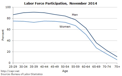
Trends in the Labor Force 1999-2014: Seniors Increase Participation, Younger Workers Withdraw

In early 2000, the civilian labor force participation rate peaked at a post-war high of 67.3 percent of the population aged 16 and over. Despite flattening out in the latter part of the decade at about 66 percent, participation rates never recovered and have steadily fallen since the onset of the Great Recession. At 62.8 percent as of November 2014, labor force participation is now at its lowest level since 1978.

Some of this fall is clearly demographic. Workers are much less likely to have or search for a job once near or past retirement age, as seen in Figure 1.

Figure 1:

Thus, the aging of the baby boom generation has reduced the size of the labor force. On the other hand, retirement-age workers are participating at a much higher rate than before. In small part, this is because baby-boomers have reduced the average age of those 65 and over. However, labor force participation in the older population has been rising for some time, as seen in Figure 2.

Figure 2:

“Mumbo-Jumbo” Mumbo-Jumbo

Today, Cato’s Alan Reynolds took a few bizarre shots from the pages of the Wall Street Journal. In particular, Reynolds it calls “far-fetched” that incomes of the middle class have stagnated for decades.

First, he asserts “The average income for the bottom 90% is not a decent proxy for the median nor even a decent measure of household income." This is clearly indefensible as a check of the numbers at Reynolds’ source demonstrates. Here, we see the average of the bottom 90 percent and the median compared for both before-tax and after-tax household income.

(Source)

Over Reynolds’ chosen 1984-2007 period, median before-tax income fell 0.05 percent per year relative to the bottom 90 percent and median after-tax income rose less than 0.01 percent per year relative to the bottom 90 percent. Obviously, such differences are in no way meaningful.

Next, Reynolds argues that median after-tax (and transfer) measures better describe the evolution of middle-class incomes than does pre-tax and transfer “market income.” However, the comparatively higher rate of growth in after-tax income simply reflects the government attempting to compensate households for the broad stagnation of income. If the median household is better off in 2007 than 23 years prior it is because we have recognized that wages have fallen and households have had to work much more to maintain a modest 0.5 percent annual increase in pre-tax income. We have increased transfers and cut taxes in order to help those households to share in the increased productivity of the economy.

It is also worth noting that much of the increased transfers which make up the wedge between market and pre-tax incomes have come as a result of a broken health-care system. The government now pays health providers considerably more and yet life expectancy for those in the bottom half of the income distribution has grown so slowly that such workers may enjoy shorter– not longer– retirements. It is not so obvious that such increases in payments contribute to growth in household income.

It is no surprise then that real per-person consumption has grown faster than median pre-tax household income. Not only does this conflate the median with the overall average— it ignores that household savings rates have declined considerably over the decades in question. In 1989, the median net wealth of households headed by someone aged 45-54 was \$177,300 compared to only \$105,400 in 2013. Even that does not consider the simultaneous decline in defined-benefit pensions held by such households.

The middle class may still appear middle class because households have dedicated more time to work, received increased assistance from the government, and accumulated considerably less wealth than the previous generations; such measures merely hide the obvious stagnation.